
To generate back-scattered light, a DTS unit launches a short pulse of light into an optical fibre. The forward propagating light generates Raman backscattered light at two new wavelengths, from all points along the fibre (Figure 1). The wavelengths of the Raman backscattered light differ from the forward propagating light and are named Stokes and anti-Stokes.

The amplitudes of the Stokes and anti-Stokes light are monitored by the DTS unit and the spatial localisation of the backscattered light is determined through knowledge of the propagation speed inside the fibre. The determination of the source of a light signal by measuring the time between the injection of a light source and the detection of a backscattered signal is the fundamental principle of OTDR. The amplitude of the Stokes light is very weakly dependent on temperature, while the amplitude of the anti-Stokes light is strongly dependent on temperature. The temperature at each sampling location is calculated by taking the ratio of the amplitudes of the measured anti-Stokes and Stokes light.
Raman is the weakest of the backscattering effects. Therefore, backscattered light from many pulses must be collected and stacked to get a useful signal from which temperature can be derived above the noise of the system. The laser pulse frequency is in the kHz range for most DTS systems. Note that as the distance to be sensed increases the pulse frequency must decrease to account for the longer time it takes light to travel in the optical fibre; a new pulse cannot be launched until the backscattered light from the previous pulse has been detected (i.e, light from two pulses cannot be present in the fibre at the same time).
A pulsed laser
The laser wavelength and pulse repetition rate must be optimised for the target measurement range (Figure 2). Wavelengths of light that experience low attenuation in optical fibre (e.g. 1550 nm) are more suitable for long range systems. Wavelengths of light that experience higher attenuation in optical fibre are optimal for shorter ranges (e.g. 1064 nm) because a stronger backscattered light signal is generated. The pulse width, or duration, must be optimised for the target spatial resolution (shorter pulse widths provide better spatial resolution).
Optoelectronic detectors
The gain and bandwidth of detectors used to measure the backscattered light signals must be optimised for the target Signal-to-Noise (SNR) and spatial resolution.
Data acquisition card
The system must be capable of spatially distributing the backscattered signal by accounting for the time of flight of the light and the sampling frequency must be specified for the target spatial resolution. The linearity of the signal digitisation circuitry is essential for accurate temperature estimation.
Optical fibre
Fibre properties must be conducive to meaningful DTS measurements with the chosen system configuration and the target application.

Fibre optic sensors, like DTS, that use the fibre directly for measurement are known as intrinsic fibre optic sensors since no other components are needed along the optical fibre. Optical fibre selection is therefore an important consideration in distributed sensing because the light that is essential for obtaining measurements experiences wavelength-dependent exponential attenuation with distance travelled through the fibre, according to Beer’s Law (also known as the Beer-Lambert law).
Optical fibres function as waveguides due to total internal reflection. Snell’s Law of Refraction describes how light is bent or refracted when it travels through two isotropic, homogeneous media with different indices of refraction n1 and n2:

where θ1 and θ2 are the angles of incidence and refraction, respectively. When light travels from a medium of greater refractive index into a medium with a lower index (n1>n2) with an incident angle greater than a critical value θcrit, Equation 1 is no longer valid as it would require sinθ2 to be greater than 1 (sinθ2>1). In this case, the light is not refracted and is instead reflected into the medium having the greater refractive index; this phenomenon is known as total internal reflection. The critical angle θcrit is given by


Optical fibres are constructed of silica (SiO2) glass and have two primary components: the core and the cladding. The core and the cladding have different indices of refraction that are chosen to maximize the total internal reflection by minimizing the normal critical angle, allowing light to travel for kilometers with minimal attenuation (Figure 3).

The core is therefore the central component of an optical fibre in which most of the light travels. The silica in the core is often doped with germanium dioxide (GeO2) or aluminium dioxide (Al2O3) to slightly increase the refractive index of the core relative to the cladding.
The optical fibres used for distributed sensing are of two main types: multimode or singlemode (Figure 4). To mechanically strengthen and protect the fragile silica core/cladding, a primary coating is applied. Use of different materials as the primary coating allow for optical fibre installations from standard to extreme temperature ranges, as listed in Figure 4.

The refractive index of the core is on the order of 1% greater in magnitude than that of the standard 125 μm diameter cladding (figure 5). The cross-section of most MM fibres also have a graded index (GI), meaning the transition in refractive index is gradual between the core and the cladding.

When an initial pulse of laser light is emitted into an optical fibre, the main mode of light propagation is along the central fibre axis. However, some light may enter the fibre at an angle to its centerline, resulting in internal reflections that cause the light to have a zig-zag or spiral path through the fibre. In this case, the optical path of some of the light rays will be longer than others and will arrive at a specific point along the fibre after the main mode light. GI MM fibres minimize this effect by allowing non-main modes of light to travel faster (due to a slightly lower index of refraction near the edge of the fibre) and better match the arrival time of main mode light at a specific point along a fibre.
Multimode 50/125 μm (core diameter/cladding diameter) GI fibres are most commonly used in DTS, as well as for most high bandwidth optical fibre communication links. Due to the substantially greater cross-sectional area, the amount of light that can be coupled into and then internally reflected in the core of a MM fibre is higher than in a SM fibre, resulting in a better signal-to-noise (SNR) ratio and resolution performance for MM DTS systems. The greater cross-sectional area minimizes core alignment mismatch resulting in less light lost at splices and mechanical connectors in the optical fibre.
Singlemode optical fibres are characterised by a small core of approximately 9 μm in diameter, which avoids modal dispersion by allowing light to propagate in only one mode. The cladding, like multimode fiber, is most often 125 μm in diameter. The much smaller diameter of singlemode fibres allows much less light to be coupled into the fibre, increasing the challenge of obtaining meaningful measurements from the Raman scattering signal.
Singlemode fibres are most commonly used for distributed acoustic or strain sensing, as these systems rely on the Rayleigh scattering signal, which is orders of magnitude more intense than the Raman scattering signal. Singlemode fibers are typically only used for DTS measurements in retrofit applications where no multimode fibre is available.
This is due to the interaction of the light with the glass, whose refractive index n is around 1.5 (compared to 1 in vacuum), and is related to v according to:

During this time, the light in the fibre, propagating at constant speed v[m/s], covers a distance ∆z (Figure 6) according to:

For example, a pulse of Δt=10 ns, travelling at v=2x10⁸ m/s, has a distance extension of Δz=2 m.

In a DTS system, backscattered light returns to the source point, where it is detected, along the same path as the incident light and with a very similar velocity to that of the incident light pulse. An incident pulse of time duration Δt (i.e. distance extent ∆z) generates a backscatter signal that is effectively the average backscatter light of a distance extent Δz/2.
The factor 1/2 comes from the fact that the incident pulse and backscatter light travel in opposite directions. The resulting temperature information is an average over the distance extent of the backscatter light signal. Therefore, the incident pulse width has a direct impact on the spatial resolution of the DTS.
| Incident pulse time duration ∆t [ns] | Incident pulse distance extent ∆z [m] | Backscatter distance extent ∆z/2 [m] |
|---|---|---|
| 1.25 | 0.25 | 0.125 |
| 2.5 | 0.5 | 0.25 |
| 5 | 1 | 0.5 |
| 10 | 2 | 1 |
TABLE 1: Typical pulse durations Δt for DTS systems, with corresponding lengths Δz and sampling resolutions Δz/2. Velocity v of light in glass is assumed to be ~2 x10⁸ [m/s] .
 Where the speed v of the traveling light pulse is given by Equation 3 (~2.108 [m/s]) and t=t1–t0.
Therefore, a light signal detected with a measured travel t=100 ns is correlated with a source 10 m away from the DTS interrogator, while a light signal detected at time t=10 µs correlates to a source 1 km away.
The determination of the distance to an optical signal source by timing the interval between emission of an optical signal and the detection of the backscattered or reflected signal is the basic principle of optical time domain reflectometry (OTDR).
Where the speed v of the traveling light pulse is given by Equation 3 (~2.108 [m/s]) and t=t1–t0.
Therefore, a light signal detected with a measured travel t=100 ns is correlated with a source 10 m away from the DTS interrogator, while a light signal detected at time t=10 µs correlates to a source 1 km away.
The determination of the distance to an optical signal source by timing the interval between emission of an optical signal and the detection of the backscattered or reflected signal is the basic principle of optical time domain reflectometry (OTDR). When light travels through an optical fibre, most of the photons are scattered elastically by silica molecules in the fibre that are much smaller than the wavelength of light in a process called Rayleigh scattering.
In Rayleigh scattering no energy is exchanged between the photons and the scattering molecules, so the wavelength of the scattered light is the same as that of the incident light. A small proportion of incident photons, however, are inelastically scattered through the processes of Raman and Brillouin scattering.
Raman scattering is due to interactions between incident photons and vibrational molecular states that result in excitation events. Unlike Rayleigh scattering, Raman scattered photons have wave properties that differ significantly from the incident light. If an electron excited by an incident photon relaxes into an energy state greater than its initial state, a photon with less energy than the incident light is emitted (the molecule gains energy from the interaction).
If the molecule loses energy in the collision however, the scattered photon will have a higher energy (shorter wavelength) than the incident photon. These two possible outcomes of an interaction result in two spectral features in the backscattered light, referred to as the Stokes (S) and anti-Stokes (aS) bands, with wavelengths above and below that of the incident light (figure 7).

The Stokes and anti-Stokes bands are symmetrical about the wavelength of the Rayleigh scattered light because they correspond to the energy difference between the same two upper and lower energy states within the scattering molecule (Figure 8). In optical fibre glass the typical wavelength shift of the Raman bands is ±~50 nm around the Rayleigh peak, which coincides with the wavelength of the emitting laser source (1064 or 1550 nm in DTS systems).

The intensities of the Stokes and anti-Stokes signals differ because the intensity depends on the relative populations of energy levels in the fibre molecules, which is temperature dependent. At thermal equilibrium, most of the molecules in a material are at a lower energy state and will absorb energy from incident photons, leading to more transitions that result in Stokes emissions than anti-Stokes emissions. The intensity of the anti-Stokes signal is therefore highly temperature dependent and the Stokes scattering signal is typically more intense.
In addition to the Rayleigh and Raman backscatter signals, a third backscattered signal, Brillouin scattering, is due to the interaction between photons and physical variations in the fibre material. Brillouin backscatter signal is the main effect that DSTS systems rely on, as this scattering mechanism is mediated by the index of refraction of the material, which, for clear materials, changes when the material experiences deformation. Material deformation varies with temperature, so Brillouin scattering is somewhat temperature dependent.
Incident photons may gain or lose energy when interacting with variations in the material, so as in Raman scattering, both wavelength upshifted and downshifted Brillouin bands are observed. Rayleigh scattering can also depend on variations in the scattering material, but such scattering is due to random fluctuations rather than the correlated fluctuations that cause Brillouin scattering. The wavelengths of the two Brillouin bands vary similarly with temperature and strain.
The wavelengths of laser light used in DTS applications are selected due to the attenuation of light in optical fibre. Light travelling in optical fibre experiences exponential attenuation with distance according to the Beer-Lambert Law, which relates the gradual loss of light with distance traveled to the refractive properties of the transmitting material. Attenuation is wavelength dependent, and the Stokes and anti-Stokes signals therefore experience different losses (Figure 9).

The wavelengths of emitted laser light in DTS systems are therefore chosen for their relatively favorable positions in the spectrum of attenuation of light in an optical fibre. 1064 nm is in the middle of a monotonic and almost linearly decreasing section of the attenuation spectrum, whereas 1550 nm corresponds to the absolute minimum of attenuation. The greater attenuation around 1064 nm (particularly for the anti-Stokes signal) makes DTS systems emitting light at this wavelength preferable for shorter length fibres, while systems with laser sources emitting at 1550 nm are mainly used for long-range applications.
The intensity of the Raman backscattered signal, composed of Stokes and anti-Stokes signals, due to light emitted through an optical fibre in a DTS system depends on the populations of quantum states within the fibre molecules.
The population of quantum states is temperature dependent, so temperature can be derived from the measured Raman scattering signal. The intensity of the photons backscattered in the anti-Stokes band increases with higher temperature, and vice versa. The Stokes signal is much less sensitive to temperature and is used for reference to quantify the variations in anti-Stokes backscatter along the optical fibre. The temperature T [K] at distance z [m] along the physical fibre is therefore determined from the ratio of the intensities of the Stokes IS and anti-Stokes IaS signals.
A widely accepted (Dakin et al., 1985) formulation of the mathematical relation is:

where
γ [K] depends on the distribution of quantum states and is a system constant fixed by manufacturing. γ quantifies the shift in energy between the photons travelling at the wavelength of the incident light and the backscattered Raman photons. (γ=ħΩ/k with ħ being Planck’s constant, Ω is the difference in frequency between the incoming laser pulse and the backscattered Stokes radiation, and k is Boltzmann’s constant.)
K is a dimensionless calibration parameter related to the temperature offset that accounts for the efficiency of the DTS components which are common factors for all the measured traces (e.g. laser optical power, efficiency of the photodiodes converting the backscattered light into electrical signal, electronic circuits).
∆α [m-1] is the differential loss calibration parameter that accounts for the difference in attenuation between the Stokes and anti-Stokes signal due to their differing wavelengths. ∆α is often expressed in [dB/km].
z [km] is the fibre distance. z=0 at the DTS instrument, though a distance offset can be specified when configuring data collection.
IS(z) and IaS(z) are the Stokes and anti-Stokes (respectively) signal amplitudes over distance.
γ, K and ∆α must be determined through DTS system calibration in order to obtain accurate distributed temperatures from Equation 7.
Each temperature measurement provided by a DTS system is averaged over a specified length increment, so the sensor output response to a change in temperature along the fibre is somewhat blurred at the edges of the change. The spatial resolution of a DTS system is therefore determined by applying a step change in temperature between two adjacent lengths of fibre (10 m or more) and determining the distance needed to capture between 10% and 90% of the variation (figure 10).

Typically, a temperature step of about 30°C is applied. The 10%-90% definition of spatial resolution is appropriate for determining the degree to which a transition can be reproduced in the sensor output.
It is important to note that different DTS manufacturers may apply different definitions, e.g. defining the sampling resolution as the spatial resolution, varying the amplitude of the step change in temperature, and/or accounting for another percentage of detection (e.g. between 20% and 80%). Extra care should be taken in reading the specifications of a DTS system to be aware of the definition of spatial resolution that is being applied.
The temperature distribution indicated by DTS data is the convolution of the sensor’s spatial response with the true spatial distribution of temperature. If the temperature features are finer than the spatial resolution of the sensor, the details of temperature variations along the fibre will be unresolvable.
If there is a hot spot (or a cold spot) along the fibre with an extent smaller than the spatial resolution, the temperature corresponding to the center of the hot spot will be lower than the actual value (Figure 11). The spatial resolution, together with the range, determines the number of independently resolvable points that can be measured by the system.

The optical interrogator in a DTS system must not trigger a light pulse until the previously emitted pulse has travelled to the end of the optical fibre and the back–scattered light has returned to the detector from every scattering point along the entire length of the fibre. If pulses are emitted any faster, the backscatter from each pulse will overlap at the detector and the data cannot be correlated with location along the fibre. A DTS system’s range is therefore the maximum length of fibre that can be measured, which dictates the maximum pulse repetition rate.
This is mathematically shown by assuming that the emitted laser light and the backscattered Stokes and anti-Stokes bands all travel at the same speed v such that the minimum time ∆t between triggers can be approximately determined as

where L is the total length of the fibre and the speed of light in the fiber v=c/n (Equation 3). This leads to a launch repetition rate R:

which is inversely proportional to the maximum optical fibre length to measure. For example, if L=5 km and n=1.5, the minimum time between triggers would be ∆t=5 μs, and therefore R=20 kHz (Table 2).
| Range (km) | Max pulse rep rate (kHz) |
|---|---|
| 5 | 20 |
| 10 | 10 |
| 15 | 6.7 |
| 20 | 5 |
| 25 | 4 |
| 30 | 3.3 |
| 35 | 2.9 |
Table 2: Maximum pulse repetition rate in kHz for different maximum measurement ranges.
The temperature resolution (e.g. 0.01 °C or 0.1 °C) and is an indicator of the precision, or repeatability, of a temperature measurement along the fibre. Temperature resolution degrades exponentially along a fibre because the backscattered signal used to determine temperature is increasingly attenuated with fibre distance.
The temperature resolution σT(x) of a DTS system along a length x of optical fibre is assessed as the standard deviation of the N consecutive samples defining the section x:

where T(x) is the temperature array and
![]()
is the average temperature for each considered section x.
The temperature resolution for a section x is typically defined by considering N=10 consecutive spatial samples. The temperature resolutions of consecutive sections x are then calculated by applying a moving window along the fibre. So for a measurement with 25 cm spatial sampling, the rolling window, centered on the measurement location, is 2.5 m long; In the case of 1 m spatial sampling, the rolling window is 10 m long.
For Equation 10 to reflect the true temperature resolution, it is assumed that the temperature is constant within the rolling window so that only the noise variation is taken into account. This is an important consideration, particularly when analysing field data where real temperature features along the fibre could mask the temperature resolution estimation by adding unwanted feature variation to the noise variation estimation.
If a more precise estimate of resolution is needed, a fitting function is used to determine the final temperature resolution along the fibre. The temperature resolution degrades exponentially over distance as the optical signal propagates following the Beer-Lambert Law. Therefore, a fitting function of the form

is used to estimate the final resolution function with distance (z is the fibre position, a and b are fitting parameters). In Figure 12, an example of σT(x) is shown in red and the exponential fit σT(z) in blue.

The launch repetition rate, or the number of pulses a DTS system can launch per second, has a significant impact on the temperature resolution, as well as the other performance factors. As the repetition rate increases, so does the number of samples that can be averaged per second. The measurement time defines the time required to obtain readings for all points along the sensing fibre to achieve the required temperature resolution.
Therefore, averaging generates a reduction of the noise floor equal to the square root of the number of samples averaged. This has a direct translation into the temperature resolution of the DTS. The temperature resolution of a DTS system improves by averaging more measurements in time (Figure 13).
Generally, from a known temperature resolution σm of a measurement of duration m, the temperature resolution σn of a measurement of any duration n (not necessarily a multiple of m) can be found as:


The subsequent change in temperature resolution follows similarly from Equation 11. The temperature resolution at a fixed spatial sample along the fibre, for different maximum fibre lengths L1 and L2 is therefore given by:

As the fibre length increases, total attenuation increases with distance and subsequently the temperature resolution degrades. The temperature resolution is degraded because as fibre length increases, the maximum possible pulse repetition frequency decreases.
For a fixed measurement time, fewer samples are collected and averaged. Use of longer width pulses and wider sampling intervals however can result in acceptable temperature resolution for measurements using longer fibres.
The terminology often used for distributed systems varies from that of conventional point transducers. In properly configured DTS systems, accuracy is constant with fibre distance and is defined as the difference of the average value of the measured temperature profile from the actual temperature, while temperature resolution is the spread in the average temperatures measured (Figure 14).
Accuracy depends upon numerous parameters affecting the measurements, including the environmental conditions of the acquisition unit and the stability of the measurements. Typically, the measurement resolution defines the smallest temperature step the unit can measure and is mainly affected by the optical pulse energy, noise in the photoreceivers, and analogue electronic front-end bandwidth. The magnitude of both the accuracy and resolution contribute to the measurement uncertainty or error of the measurements.

Accurate DTS temperature measurements at a distance z (m) depend on the ability of the instrument to measure the intensities of the backscattered Stokes and anti-Stokes signals, which is impacted by physical parameters of the DTS system: γ, K, and ∆α. The determination of these three parameters defines the precision and accuracy of a DTS system’s temperature measurements and can be explicitly calculated or resolved, depending on the configuration of the DTS system. Implicit determination of these calibration parameters is not the norm, but, for some applications, doing so can provide additional configuration flexibility and allow for improved temperature resolution.

DTS systems can function with a variety of configurations of optical fibre, which affect how the system resolves temperature. DTS units are designed to allow for data collection from single or multiple fibres, which are connected to various emission/detection channels. The two most basic configurations are referred to as single-ended and double-ended (Figure 15). In a single-ended configuration, laser pulses are input and backscattered light is measured at the same end of the fibre, which is connected to one channel of the DTS. In a double-ended configuration, the fibre extends from the DTS and is looped back so that each end of the fibre is connected to differing detection channels. Laser pulses are input and monitored from both ends of the fibre (or both channels), alternating sides during each measurement interval.
Explicit calculation of γ, K, and ∆α for any system configuration relies on three independent comparisons of three observed reference temperatures, usually with two as close as possible to the laser source where light attenuation with distance is negligible (to calibrate γ and K, respectively) and one at the far end of the optical fibre (to calibrate ∆α). However, in practice, γ is a fixed value determined by the instrument manufacturer and has proven to be insensitive to the main factors affecting the other parameters, so it is reasonable to assume that it is constant in time. Therefore, for most applications, the differential attenuation ∆α and temperature offset K parameters are the parameters that must be determined, and they are derived differently depending on the DTS system configuration. Calibration procedures can be greatly simplified by the capabilities of a given DTS unit and the use of specific cable configurations which can reduce the number of external, independent temperature comparisons needed and the amount of data post-processing required, without a decrease in accuracy.
Attenuation caused by these various fibre features may also vary with fibre temperature, resulting in temporal variations in attenuation. In the case that attenuation is uniform along a fibre, ∆α can be determined through calibration based on independent temperature measurements at two points along the cable and the temperature can be determined from Equation 6, assuming all other parameters are known. ∆α can also be set at a fixed, constant value (e.g. 0.1 dB/km) according to the specifications of the optical fibre being used. In most DTS applications however, attenuation varies along the cable due to combinations of some of the irregularities mentioned. In this case, all attenuating effects between the DTS unit at z’=0 and the sample location z’=z must be combined. In this case, the temperature equation takes the form:

The integral
![]()
has the unit of dB, so must be scaled by ln(10)/10000 to change the units from dB to linear.
Calibration measurements necessary to determine differential attenuation in DTS systems can be achieved by holding a section or, ideally, two sections of optical fibre at known, constant temperatures. Typically, sections of optical fibre are coiled and placed into temperature-controlled baths inside insulated containers such that the fibre does not contact the container and experience temperature variations.
Since temperature is averaged over a length of fibre, the section of fibre in the bath should be at least 10–25 m long and bath temperature should be continuously and independently monitored for reference; a 100 Ohm platinum resistance thermistor (Pt100) is the standard sensor used. If a fibre is composed of several joined sections of fibre, each section must be individually calibrated.

Most DTS systems include automated calibration algorithms for correcting for the differential attenuation using different system configurations. These so-called differential loss corrections terms are known as fixed value, temperature matching, external probe, or double-ended. Fixed value, temperature matching, and external probe options are most commonly used for single-ended fibre configurations.
In a DTS system with a single-ended configuration, both the temperature offset and differential attenuation parameters must be determined through calibration unless a differential loss correction term can be specified in the DTS system configuration. Proper differential loss correction is required to maintain accuracy with distance from the DTS unit for single-ended measurements.
To determine the double-ended differential loss correction term, laser pulses are launched into the fibre from alternating ends of the fibre (e.g., a pulse is launched in the ‘forward’ direction from the end of fibre connected to Channel 1 during the first measurement period and launched in the ‘reverse’ direction from Channel 2 during the second measurement period, and so on). Following Dakin et al. (1985), the ‘forward’ laser pulse starts at z=0 and the ‘reverse’ pulse starts at z=L, with L being the length of the cable. If the temperature over a span Δz remains constant during the forward and reverse measurement periods, Equation 14 can be used to solve for the differential attenuation Δα by setting T(z)=T(L‑z) and rearranging:

The arrows (←,→) indicate whether the measurement is considered in the forward or reverse direction. By obtaining a measurement from each sample Δz along the entire length of the fibre and integrating the values, the differential attenuation ∆α at each location z can be determined. The data used is a time-average over the entire measurement period, during which it is assumed ∆α remains constant.
Longer measurement integration times and spatial averaging are used so that the value of differential attenuation obtained through calibration does not add significantly to the uncertainty of DTS temperature measurements. Since the temperature reported for each sample in a double-ended system is determined from signals travelling from both directions in the fibre, the measurements are noisiest closest to the sensor and have the least noise at the midpoint of the fibre.
Double-ended calibration uniquely and robustly corrects for differential light loss that varies over the length of the fibre. There is no requirement for the fibre to follow the same path or for fibre at a given distance from the unit on both sides of the loop to have the same temperature, though double-ended calculations do require very precise alignment of the forward and reverse signals.
Using a loop of fiber with double-ended differential loss calibration on a linear object requires the length of fibre to be doubled. Also, the interrogator must probe twice the length of an equivalent single-ended system, which may lead to decreased resolution for longer lengths of fibre.
Use of this method is mostly recommended when the fibre is located in a particularly harsh environment and is likely subject to damage-induced changes in differential loss. In other cases, it is generally advisable not to use double-ended calibration because of the complexity of the configuration required.

The temperature offset therefore has the same effect on each temperature sample (Figure 18), unlike the differential attenuation, which generally has a greater effect on samples farther from the DTS unit (Figure 16). Some of the quantities characterizing the temperature offset are sensitive to the operational temperature changes experienced by a DTS instrument which may cause the offset to vary in time.

Unless the DTS instrument can be maintained at a very stable temperature, the temperature offset must be determined for each measurement. An uncalibrated temperature offset manifests as a distant-invariant deviation from the true temperature for each sample. While this does not affect the accuracy of the measured relative changes in temperature, it does affect the accuracy of the absolute temperature measurements.
From the known value of γ and the determined value of the differential attenuation ∆α, the value of the temperature offset is easily obtained using a known temperature reference to calculate an offset for the entire data set. Typically, the temperature offset is dynamically determined within the DTS instrument using a highly accurate internal temperature reference; however, for unique applications, offset calibration using a probe and/or an external fiber reference section may be appropriate.
Use of a reference section and a probe is preferable over a single point-source measurement because this method allows for the noise in the measurement to be averaged out and improves the temperature resolution.
An external probe to determine the temperature offset can be used when the probe can be placed such that it is at the same temperature as the average temperature along a selected section of the sensing fibre. In practice, the external probe option is only used to determine the temperature offset when an insulated coil of the sensing fibre is positioned, along with the probe, near the DTS unit. When this option is chosen, the DTS ignores the internal reference and instead uses the selected external probe and reference section as the inputs into the temperature offset calculation. If the external probe option is used for both the differential loss and temperature offset calibrations, then the reference section and probe must be at different locations or temperatures in both cases.
Typically, the reference section consists of several meters of coiled optical fibre placed in a homogenous hot or cold water bath, or in a thermally isolated container. To achieve accurate calibration, the fibre temperature must be constant in space and preferably constant, or slowly varying in time, during the DTS system measurement to assure that the temperature measured by the external probe accuracy reflects that of the reference fibre.
The use of water mixers is highly recommended during calibration to avoid the generation of vertical temperature gradients within the bath. To minimally reduce the effects of heat exchange between the environment and the bath, the coil of reference cable should be placed horizontally within the bath and contact should be avoided with the walls.
The length of the reference section of cable used for calibration is not fixed, though the maximum possible optical fibre length that can be placed in the bath while following the stated guidelines is recommended.
Longer reference fibres provide more data points, and thus a more statistically robust average temperature measurement for comparison to the independent probe measurement. For example, if 10 m of optical fibre is used as a reference section with a sampling resolution of 12.5 cm, the average temperature is determined from 80 samples.
The difference between the temperatures measured simultaneously by the independent probe and by the reference fibre determines the offset, which is then added (with the appropriate sign) to all points of the DTS measurement. The offset should be calculated and corrected for each DTS measurement.
Active DTS methods are of particular use in hydrogeological and atmospheric DTS applications in which environmental properties can be determined from the measured temperature profile in time. Here we will briefly discuss only the method which makes use of a hybrid (composite) cable containing both an optical fibre used for DTS measurement and a heating element with a constant power output per meter.
The amount of thermal transport away from the cable can be determined from the measured variations in temperature along the fibre. The measured temperature response in time caused by environmental heat transport can be used to determine the thermal properties of the measurement environment, including the apparent thermal conductivity of material surrounding the fibre. Active DTS also provides a way to characterize a variety of physical properties that affect thermal conductivity, such as seepage, soil moisture, or even wind speed.
Active heating is much more common than active cooling because an electrical resistance circuit can easily be used as a linear heater in the cable. Cooling methods such as circulation of fluids or utilising refrigeration are far more challenging.
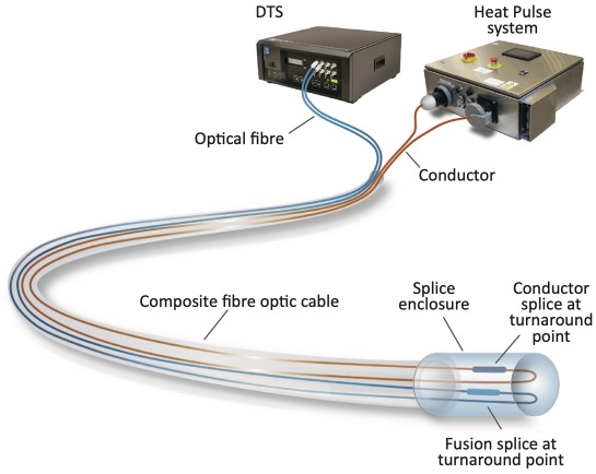
If the resistance and voltage are held constant, the power output per meter of cable is unchanging in time (figure 19). A constant power output along the cable is generally required for calculating parameters from the temperature response due to the inherent variability of many environmental factors, such as fluid flow (figure 20).
Pulse modulation of heating can be used in some cases to characterise the contrast between heated and unheated environmental conditions. The design of an active DTS system is dependent on the physical quantities that are to be derived from the measured temperature response.

Ohm’s law,

where I is the current in amperes (A) through the conductor, V is the voltage applied across the conductor in volts (V), and R is the resistance in ohms (Ω), can therefore be used to determine the voltage necessary to achieve the desired power rate per unit length in Watts per meter (W/m), where

Typical values can vary from 1–2 W/m for atmospheric measurements such as wind speed, to 10–20 W/m for geothermal wells and shallow soil monitoring (Figure 21).
The thermal properties of the environment surrounding the heated cable and the resolution of the DTS system dictate the amount of voltage necessary to apply to the conductor to achieve the desired power output and to generate a clearly detectable thermal signature.

Attenuation is a physical process independent of the resolved temperature and leads to an unavoidable degradation of temperature resolution with distance. Beer’s law describes this fundamental intrinsic fibre loss as an exponential decay with distance z of the initial (i.e. z=0) light intensity I0 according to:

where α [1/m] is the wavelength-dependent attenuation coefficient of the travelling wave and I0 is the intensity at z=0. Alternatively, α is also often expressed in [dB/km], which is related to the [1/m] value by the following relation:

For the temperature determination at a certain distance z along the optical fibre it is necessary to calculate the intensity IS(z) and IaS(z) of the Stokes and anti-Stokes backscatters, respectively. IS(z) and IaS(z) are expressed as:


where


IaS(z) and IS(z) account for the fact that the primary pulse intensity (at z=0), is attenuated at a rate αR of the incident light (same as the Rayleigh wave) at z, whereas the returning signals to z=0 experience an attenuation αaS for the anti-Stokes band and αS for the Stokes band.
The attenuation terms αaS, αR and αS differ because the wavelengths of the emitting laser source and backscattered anti-Stokes and Stokes signals are different and therefore experience different losses.
The Stokes and anti-Stokes quantum mechanical terms both contain a temperature dependence, though the anti-Stokes signal proves to have greater temperature dependency. Therefore, the Stokes band is therefore not completely insensitive to temperature variations. However, it is used as a reference and the DTS temperature information is obtained from the ratio of the Stokes and anti-Stokes intensities, as this allows simplifying the calculations:

where Δα = αS-αAS = differential attenuation [m-1] or![]()
Solving the above equation for the temperature (in Kelvin) results in:

where
![]()